With this article we want to analyze a randomized complete block design (RCBD) to show how a traditional full fixed effects model and ANOVA work.
1) Setup & data
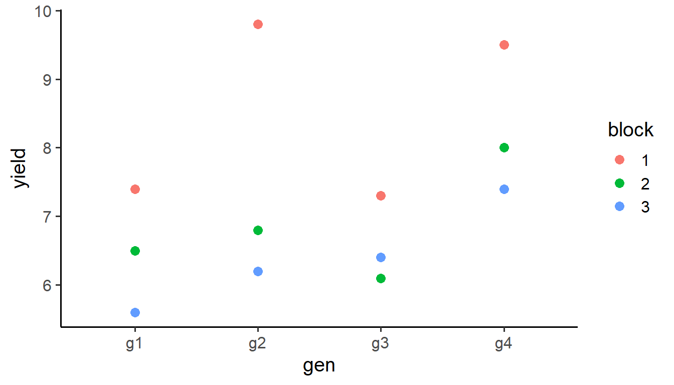
Clewer and Scarisbrick (2001) present a yield trial (t/ha) conducted using a randomized complete block design. The design included 3 blocks and 4 cultivars, resulting in 12 experimental plots.
library(tidyverse)library(emmeans)library(gt)library(kableExtra)# Read and coerce factorsdata <-read.csv("../data/example_1.csv") |>mutate(gen =as.factor(gen), block =as.factor(block))head(data)
data |>ggplot(aes(x = gen, y = yield, color = block)) +geom_point(size =3) +theme_classic(base_size =15)
Yield by genotype colored by block.
2) Linear model building blocks
We will progressively build the RCBD model using model.frame() and model.matrix() to see the design matrices explicitly, then solve normal equations. We use:
\(\boldsymbol{y} = \boldsymbol{X\beta} + \boldsymbol{\varepsilon}\): linear model
Notice that the first term, \(\left(\boldsymbol{X'X}\right)^{-1}\), corresponds to the inverse of number of observations, while the second term, \(\boldsymbol{X'y}\), gives the sum of phenotypic values.
In this example, there is only a single level, \(\mu\). Therefore, the entire expression simplifies to the sum of the phenotypic values divided by the number of observations, which is simply the mean, as shown below:
In this model, there are 3 levels (\(Block1\), \(Block2\) and \(Block3\)). Therefore, the entire expression simplifies to the sum of the phenotypic values divided by the number of observations, which is simply the mean per block.
data |>group_by(block) |>summarise(beta =mean(yield, na.rm =TRUE)) |>gt()
In this model, there are 4 levels (\(g1\), \(g2\), \(g3\) and \(g4\)). Therefore, the entire expression simplifies to the sum of the phenotypic values divided by the number of observations, which is simply the mean per genotype.
data |>group_by(gen) |>summarise(beta =mean(yield, na.rm =TRUE)) |>gt()
Let’s be careful when interpreting the coefficients and the variance of these factor coefficients. In a linear model, when you include a categorical factor like “genotype”, the model needs a baseline. In R it chooses g1 as the reference. Therefore:
The coefficient for g2 is the estimated difference between g2 and g1 (7.6 - 6.5 = 1.1).
The variance for the g2 coefficient is the uncertainty around that difference (g2 - g1).
3) Reduction-in-SS and ANOVA table
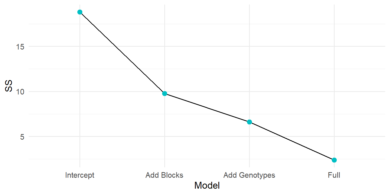
Partial Sum of Squares (SS) measures the unique contribution of a predictor variable to a model, accounting for all other variables. It is calculated by comparing the error sum of squares (SSE) of the model without the variable to the SSE of the model with it. A larger reduction in SSE indicates a greater unique contribution of that variable.
anova_dt <-data.frame(Source =c("block", "gen", "residuals"), # factors included in the modelDf =c(n_blks -1, n_gens -1, n -length(beta)), # `n - p`, where `p` is the number of coefficientsSSq =c(SSE_mu - SSE_blk, SSE_mu - SSE_gen, SSE) # differences between baseline model and nested models) |>mutate(MSq = SSq / Df,F.value = MSq / MSq[3],`Pr(>F)`=pf(q = F.value, df1 = Df, df2 = Df[3], lower.tail =FALSE),F.value =ifelse(Source =="residuals", NA, F.value),`Pr(>F)`=ifelse(Source =="residuals", NA, `Pr(>F)`) )anova_dt |>gt()
Source
Df
SSq
MSq
F.value
Pr(>F)
block
2
9.78
4.89
12.225
0.007650536
gen
3
6.63
2.21
5.525
0.036730328
residuals
6
2.40
0.40
NA
NA
Note
Why does this work? In fixed-effects ANOVA, Type-I SS for adding a factor equals the reduction in SSE between nested models. Here we use the intercept-only model as the baseline; adding block or gen reduces SSE by their respective SS.
4) Verify with lm()
mod <-lm(yield ~1+ block + gen, data = data)anova(mod)
Analysis of Variance Table

Response: yield
          Df Sum Sq Mean Sq F value   Pr(>F)
block      2   9.78    4.89  12.225 0.007651 **
gen        3   6.63    2.21   5.525 0.036730 *
Residuals  6   2.40    0.40
---
Signif. codes:  0 '***' 0.001 '**' 0.01 '*' 0.05 '.' 0.1 ' ' 1
With block and gen as factors and an intercept present, R uses treatment (baseline) coding by default. The printed beta therefore contains:
beta[1]: the intercept (no longer overall mean)
beta[2:3]: effects for non-reference blocks
beta[4:6]: effects for non-reference genotypes
You can reconstruct overall mean, genotype means, and block means as follows.
# Number of coefficients in full modeln_coef <-length(beta)# Overall mean reconstructed from coefficientsmu_recon <- beta[1] +sum(beta[2:3]) / n_blks +sum(beta[4:6]) / n_gens# Compare with the intercept-only estimatemu_recon - beta_mu[1]
[1] 7.993606e-15
5.1 Genotype means including the missing (baseline) level
# beta currently has: (Intercept), block2, block3, gen2, gen3, gen4# Create a named vector for gen effects including the reference level set to 0print(beta)