Quadratic–plateau–linear function

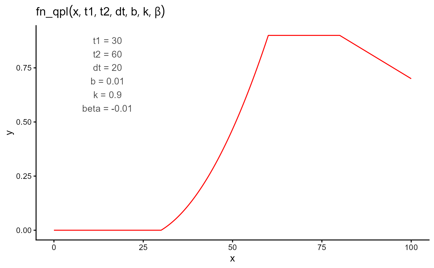
A piecewise function that models an initial quadratic increase from zero up to a plateau, maintains that plateau for a duration, and then changes linearly after the plateau ends.

Usage

fn_qpl(t, t1, t2, dt, b, k, beta)

Arguments

t

A numeric vector of input values (e.g., time).

t1

The onset time of the response. The function is 0 for all values less than t1.

t2

The time when the quadratic growth phase ends and the plateau begins. Must be greater than t1.

dt

Duration of the plateau. Defines t3 = t2 + dt and must be non-negative.

b

Linear coefficient of the quadratic growth phase.

k

The plateau value (level maintained between t2 and t3).

beta

Slope of the final linear phase after t3 (often negative).

Value

A numeric vector of the same length as t, representing the function values.

Details

The quadratic phase is parameterized so that the curve reaches exactly k at t2. Let \(\Delta = t_2 - t_1\). The quadratic coefficient \(c\) is computed internally as: $$ c = \frac{k - b\Delta}{\Delta^2}. $$

$$ f(t; t_1, t_2, dt, b, k, \beta) = \begin{cases} 0 & \text{if } t < t_1 \\ b(t - t_1) + c(t - t_1)^2 & \text{if } t_1 \le t \le t_2 \\ k & \text{if } t_2 < t \le t_3 \\ k + \beta (t - t_3) & \text{if } t > t_3 \end{cases} $$

where \(t_3 = t_2 + dt\).

The function is continuous at t1, t2, and t3. It is not differentiable at t3 unless beta = 0.

Examples

library(flexFitR)
plot_fn(
  fn = "fn_qpl",
  params = c(t1 = 30, t2 = 60, dt = 20, b = 0.01, k = 0.9, beta = -0.01),
  interval = c(0, 100),
  n_points = 2000,
  auc_label_size = 3
)