Getting started
The basic idea of this vignette is to illustrate to users how to use the flexFitR package. We’ll start with a very basic example: a simple linear regression. Although this example is not the primary focus of the package, it will serve to demonstrate its use.
1. Simple linear regression
In this example, we’ll work with a small dataset consisting of 6 observations, where X is the independent variable and Y is the dependent variable.
dt <- data.frame(X = 1:6, Y = c(12, 16, 44, 50, 95, 100))
plot(explorer(dt, X, Y), type = "xy")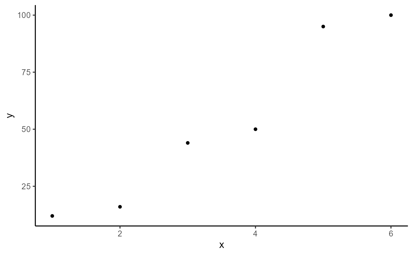
First, we define an objective function. In this case, the function
fn_lm will represent the linear regression, where b is the
intercept and m is the slope of the regression.
fn_lm <- function(x, b, m) {
  y <- b + m * x
  return(y)
}
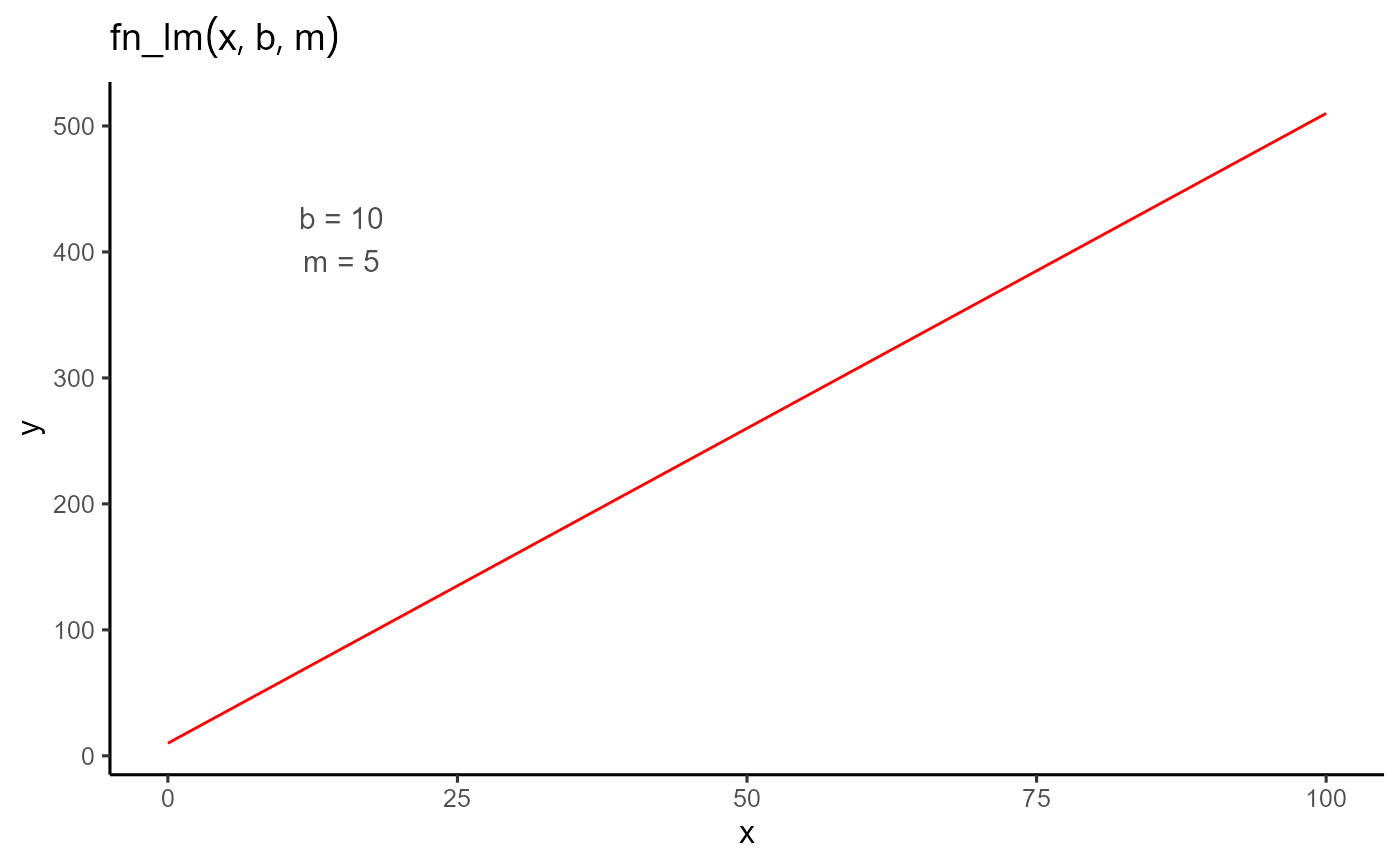
The plot_fn function, which is integrated into the
package, allows us to plot any function with the parameters provided.
This is useful for visualizing the shape of the function before fitting
the model to the data.
To fit the model, we use the modeler function. In this
function, we pass x as the independent variable, y as the dependent
variable, and then a vector of parameters where we assign initial values
to our coefficient b and coefficient m.
mod <- dt |>
  modeler(
    x = X,
    y = Y,
    fn = "fn_lm",
    parameters = c(b = -5, m = 10)
  )
mod
#>
#> Call:
#> Y ~ fn_lm(X, b, m)
#>
#> Residuals (`Standardized`):
#>     Min.  1st Qu.   Median     Mean  3rd Qu.     Max.
#> -1.18875 -0.57369 -0.03282  0.00000  0.58494  1.21753
#>
#> Optimization Results `head()`:
#>  uid     b    m sse
#>    1 -15.5 19.5 449
#>
#> Metrics:
#>  Groups      Timing Convergence Iterations
#>       1 0.3504 secs        100%   354 (id)
Once the model is fitted, we can examine the output, extract the estimated parameters, make some plots, and predict new x values.
a <- plot(mod, color = "blue", title = "Raw data")
b <- plot(mod, type = 4, n_points = 200, color = "black")
ggarrange(a, b)
#> Ignoring unknown labels:
#> • colour : "Model"
#> • fill : "Model"
#> • linetype : "Model"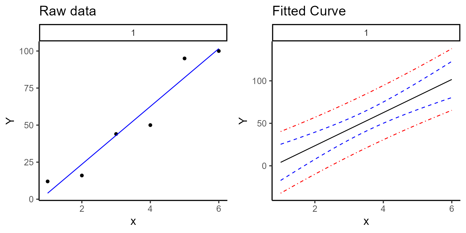
In order to get the coefficients with their variance-covariance
matrix we make use of the coef and vcov
function, which only takes the model object as an argument.
coef(mod)
#> # A tibble: 2 × 7
#>     uid fn_name coefficient solution std.error `t value` `Pr(>|t|)`
#>   <dbl> <chr>   <chr>          <dbl>     <dbl>     <dbl>      <dbl>
#> 1     1 fn_lm   b              -15.5      9.86     -1.57    0.192
#> 2     1 fn_lm   m               19.5      2.53      7.71    0.00152
vcov(mod)
#> $`1`
#>           b          m
#> b  97.21937 -22.435238
#> m -22.43524   6.410068
#> attr(,"fn_name")
#> [1] "fn_lm"
Finally, we can make predictions using the predict function, which takes the fitted model as an object and X as the value for which we want to make the prediction.
predict(mod, x = 4.5)
#> # A tibble: 1 × 5
#>     uid fn_name x_new predicted.value std.error
#>   <dbl> <chr>   <dbl>           <dbl>     <dbl>
#> 1     1 fn_lm     4.5            72.3      5.01
We can compare this with the lm function in R, which will give results similar to those obtained with our package.
Comparison with lm
mo <- lm(Y ~ X, data = dt)
summary(mo)$coefficients
#>              Estimate Std. Error   t value    Pr(>|t|)
#> (Intercept) -15.46667   9.859988 -1.568629 0.191812151
#> X            19.51429   2.531811  7.707639 0.001524882
vcov(mo)
#>             (Intercept)          X
#> (Intercept)    97.21937 -22.435238
#> X             -22.43524   6.410068
predict(mo, newdata = data.frame(X = 4.5), se.fit = TRUE)
#> $fit
#>        1
#> 72.34762
#>
#> $se.fit
#> [1] 5.010599
#>
#> $df
#> [1] 4
#>
#> $residual.scale
#> [1] 10.59133
While the previous example was fairly simple, we can consider a more
complex scenario where we need to fit not just one function, but
hundreds of functions for several groups. This can be achieved using the
grp argument in the modeler function.
Additionally, we can parallelize these processes by setting the
parallel argument to TRUE and defining the
number of cores to use.
It’s important to note that depending on the functions defined by the user, some parameters may need to be constrained, such as being required to be greater than or less than zero. In other cases, certain parameters might need to be fixed at known values. In these more complex situations, where we have many curves to fit and are working with complex functions—whether non linear regressions with specific parameter constraints or cases where some parameters are fixed for each group—modeler offers extensive flexibility.
2. Piece-wise regression
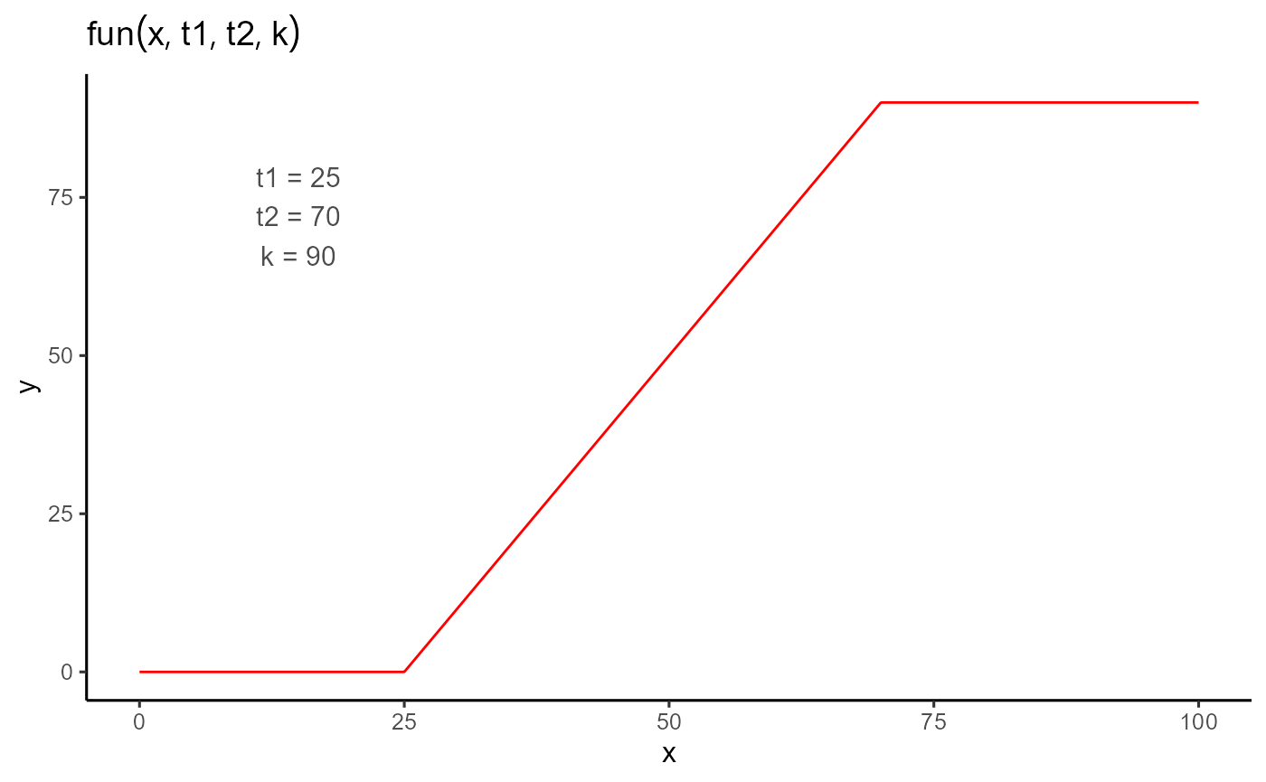
The following example, although still simple, represents a slightly
more complex function with a greater number of parameters. In this case,
we have a piece-wise regression, parameterized by t1,
t2, and k, and defined by the following
expression:
fun <- function(t, t1 = 45, t2 = 80, k = 0.9) {
  ifelse(
    test = t < t1,
    yes = 0,
    no = ifelse(
      test = t >= t1 & t <= t2,
      yes = k / (t2 - t1) * (t - t1),
      no = k
    )
  )
}
Before fitting the model, let’s take a look at the example dataset.
dt <- data.frame(
  time = c(0, 29, 36, 42, 56, 76, 92, 100, 108),
  variable = c(0, 0, 0.67, 15.11, 77.38, 99.81, 99.81, 99.81, 99.81)
)
plot(explorer(dt, time, variable), type = "xy")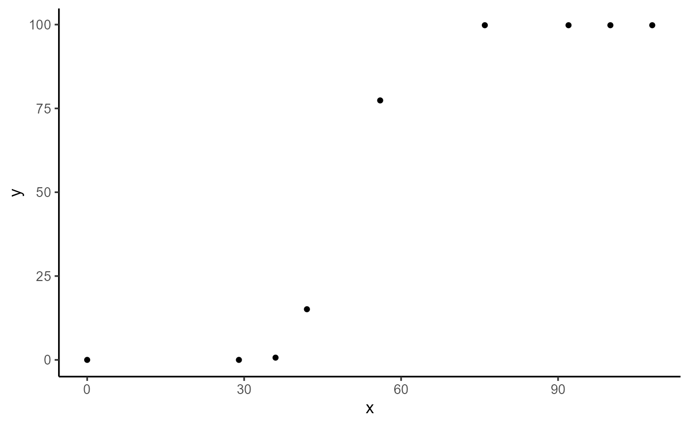
We can make a plot of the piecewise function and then fit the model
using the modeler function.
mod_1 <- dt |>
  modeler(
    x = time,
    y = variable,
    fn = "fun",
    parameters = c(t1 = 40, t2 = 70, k = 100)
  )
mod_1
#>
#> Call:
#> variable ~ fun(time, t1, t2, k)
#>
#> Residuals (`Standardized`):
#>       Min.    1st Qu.     Median       Mean    3rd Qu.       Max.
#> -1.000e-08  0.000e+00  0.000e+00  2.722e-01  0.000e+00  2.449e+00
#>
#> Optimization Results `head()`:
#>  uid   t1 t2    k   sse
#>    1 38.6 61 99.8 0.449
#>
#> Metrics:
#>  Groups      Timing Convergence Iterations
#>       1 0.4093 secs        100%   473 (id)
After fitting the model, we can examine the results, plot the fitted curve, extract the coefficients and their associated p-values, obtain the variance-covariance matrix, and make predictions for unknown values of x.
plot(mod_1)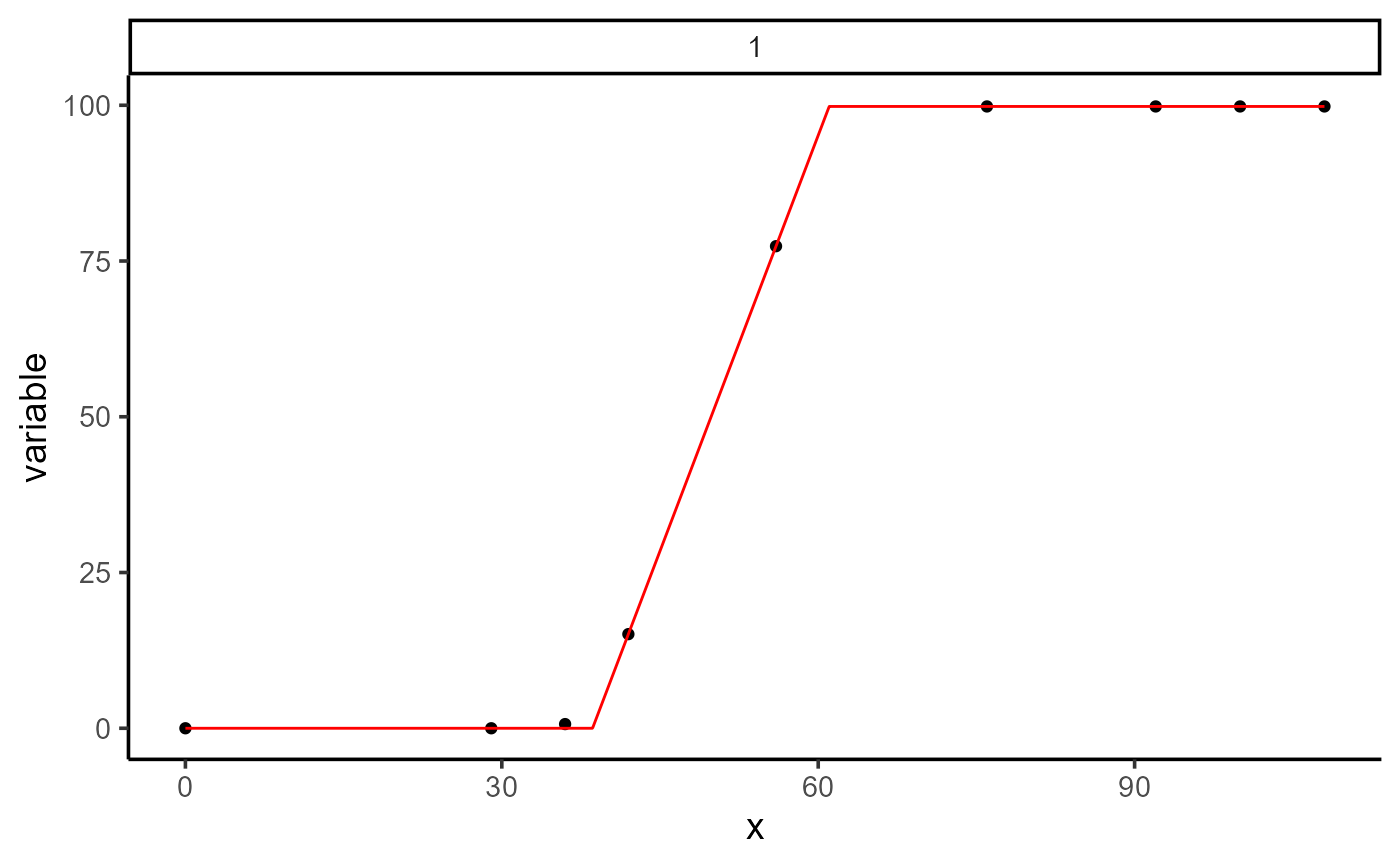
# Coefficients
coef(mod_1)
#> # A tibble: 3 × 7
#>     uid fn_name coefficient solution std.error `t value` `Pr(>|t|)`
#>   <dbl> <chr>   <chr>          <dbl>     <dbl>     <dbl>      <dbl>
#> 1     1 fun     t1              38.6    0.0779      496.   4.54e-15
#> 2     1 fun     t2              61.0    0.0918      665.   7.82e-16
#> 3     1 fun     k               99.8    0.137       730.   4.47e-16
# Variance-Covariance Matrix
vcov(mod_1)
#> $`1`
#>               t1           t2            k
#> t1  6.061705e-03 -0.002940001 1.877076e-07
#> t2 -2.940001e-03  0.008431400 4.204939e-03
#> k   1.877076e-07  0.004204939 1.870426e-02
#> attr(,"fn_name")
#> [1] "fun"
# Making predictions
predict(mod_1, x = 45)
#> # A tibble: 1 × 5
#>     uid fn_name x_new predicted.value std.error
#>   <dbl> <chr>   <dbl>           <dbl>     <dbl>
#> 1     1 fun        45            28.5     0.223
Comparison with nls
mod_nls <- dt |>
  nls(
    formula = variable ~ fun(time, t1, t2, k),
    start = c(t1 = 40, t2 = 70, k = 100),
    algorithm = "default"
  )
summary(mod_nls)
#>
#> Formula: variable ~ fun(time, t1, t2, k)
#>
#> Parameters:
#>    Estimate Std. Error t value Pr(>|t|)
#> t1 38.60286    0.07786   495.8 4.54e-15 ***
#> t2 61.04288    0.09183   664.7 7.82e-16 ***
#> k  99.81000    0.13676   729.8 4.47e-16 ***
#> ---
#> Signif. codes:  0 '***' 0.001 '**' 0.01 '*' 0.05 '.' 0.1 ' ' 1
#>
#> Residual standard error: 0.2735 on 6 degrees of freedom
#>
#> Number of iterations to convergence: 4
#> Achieved convergence tolerance: 3.927e-06
coef(mod_nls)
#>       t1       t2        k
#> 38.60286 61.04288 99.81000
vcov(mod_nls)
#>               t1           t2             k
#> t1  6.062452e-03 -0.002940973 -6.025873e-13
#> t2 -2.940973e-03  0.008433026  4.205209e-03
#> k  -6.025873e-13  0.004205209  1.870417e-02
predict(mod_nls, newdata = data.frame(time = 45))
#> [1] 28.45357
As we can see, we get very similar results when compared to
nls.
Finally, we will illustrate how to provide different initial values to the function when dealing with multiple groups, and we will also show how to fix some parameters of the objective function.
Providing Initial values
In this example, we don’t have a grouping variable. However, by
default, the function assigns a unique identifier (uid) to
the dataset. Because of this, we need to specify uid = 1
for the initial values and fixed parameters. If there is only one group,
you only need to modify the parameters argument accordingly. This
approach is primarily for illustrative purposes.
init <- data.frame(uid = 1, t1 = 20, t2 = 30, k = 0.8)

mod_2 <- dt |>
  modeler(
    x = time,
    y = variable,
    fn = "fun",
    parameters = init
  )
mod_2
#>
#> Call:
#> variable ~ fun(time, t1, t2, k)
#>
#> Residuals (`Standardized`):
#>       Min.    1st Qu.     Median       Mean    3rd Qu.       Max.
#> -1.000e-08  0.000e+00  0.000e+00  2.722e-01  0.000e+00  2.449e+00
#>
#> Optimization Results `head()`:
#>  uid   t1 t2    k   sse
#>    1 38.6 61 99.8 0.449
#>
#> Metrics:
#>  Groups      Timing Convergence Iterations
#>       1 0.4087 secs        100%   567 (id)
coef(mod_2)
#> # A tibble: 3 × 7
#>     uid fn_name coefficient solution std.error `t value` `Pr(>|t|)`
#>   <dbl> <chr>   <chr>          <dbl>     <dbl>     <dbl>      <dbl>
#> 1     1 fun     t1              38.6    0.0779      496.   4.54e-15
#> 2     1 fun     t2              61.0    0.0918      665.   7.82e-16
#> 3     1 fun     k               99.8    0.137       730.   4.47e-16
Fixing parameters
fix <- data.frame(uid = 1, k = 98)

mod_3 <- dt |>
  modeler(
    x = time,
    y = variable,
    fn = "fun",
    parameters = c(t1 = 40, t2 = 70, k = 100),
    fixed_params = fix
  )
mod_3
#>
#> Call:
#> variable ~ fun(time, t1, t2, k)
#>
#> Residuals (`Standardized`):
#>    Min. 1st Qu.  Median    Mean 3rd Qu.    Max.
#>  0.0000  0.0000  0.4815  0.6316  1.3008  1.3008
#>
#> Optimization Results `head()`:
#>  uid   t1   t2  sse  k
#>    1 38.6 60.6 13.6 98
#>
#> Metrics:
#>  Groups      Timing Convergence Iterations
#>       1 0.3306 secs        100%   313 (id)
coef(mod_3)
#> # A tibble: 2 × 7
#>     uid fn_name coefficient solution std.error `t value` `Pr(>|t|)`
#>   <dbl> <chr>   <chr>          <dbl>     <dbl>     <dbl>      <dbl>
#> 1     1 fun     t1              38.6     0.396      97.5   3.15e-12
#> 2     1 fun     t2              60.6     0.429     141.    2.34e-13
plot(mod_3)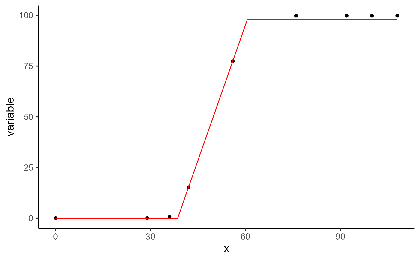
performance(mod_1, mod_2, mod_3)
#>   fn_name uid df nobs p logLik   AIC  AICc   BIC Sigma   SSE  MAE  MSE RMSE R2
#> 1   fun_1   1  4    9 3   0.72  6.56 16.56  7.35  0.27  0.45 0.07 0.05 0.22  1
#> 2   fun_2   1  4    9 3   0.72  6.56 16.56  7.35  0.27  0.45 0.07 0.05 0.22  1
#> 3   fun_3   1  3    9 2 -14.61 35.23 40.03 35.82  1.39 13.55 0.88 1.51 1.23  1
This vignette provided a basic introduction to using the flexFitR package, starting with simple examples such as linear regression and piecewise regression. The goal was to demonstrate the fundamental features and flexibility of the package. However, more complex situations can arise when working with high-throughput phenotypic (HTP) data, which involve multiple groups, parameter constraints, and advanced modeling scenarios. These more complex situations are illustrated in the other vignettes, which use real HTP data to showcase the full capabilities of the flexFitR package.
