Modeling plant emergence and canopy growth using UAV data • flexFitR

This vignette demonstrates piecewise regression using canopy data derived from UAV imagery to estimate two key parameters:

t1: days to plant emergence.
t2: days to reach maximum canopy.

The data are from the University of Wisconsin-Madison potato breeding program, specifically for a partially replicated experiment. The UAV images were collected in 2020 and processed in 2024.

Loading libraries

library(flexFitR)
library(dplyr)
library(kableExtra)
library(ggpubr)
library(purrr)

1. Exploring data

We begin with the explorer function, which provides basic statistical summaries and descriptive statistics, as well as visualizations to help understand the temporal evolution of each plot.

data(dt_potato)
explorer <- explorer(dt_potato, x = DAP, y = Canopy, id = Plot)

names(explorer)
#> [1] "summ_vars"      "summ_metadata"  "locals_min_max" "dt_long"       
#> [5] "metadata"       "x_var"

p1 <- plot(explorer, type = "evolution", return_gg = TRUE, add_avg = TRUE)
p2 <- plot(explorer, type = "x_by_var", return_gg = TRUE)
ggarrange(p1, p2)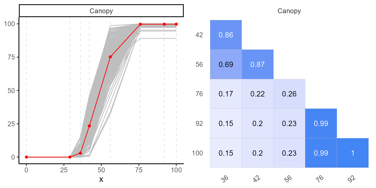

plot corr

To see more about the type of plots visit plot.explorer().

var	x	Min	Mean	Median	Max	SD	CV	n
Canopy	0	0.00	0.00	0.00	0.00	0.00	NaN	196
Canopy	29	0.00	0.00	0.00	0.00	0.00	NaN	196
Canopy	36	0.00	2.95	1.84	15.09	3.22	1.09	196
Canopy	42	0.76	23.38	22.91	46.23	9.31	0.40	196
Canopy	56	32.51	75.20	74.96	98.62	12.26	0.16	196
Canopy	76	89.06	99.72	100.00	100.00	1.04	0.01	196
Canopy	92	89.06	99.75	100.00	100.04	1.02	0.01	196
Canopy	100	89.06	99.75	100.00	100.04	1.02	0.01	196

2. Regression Function

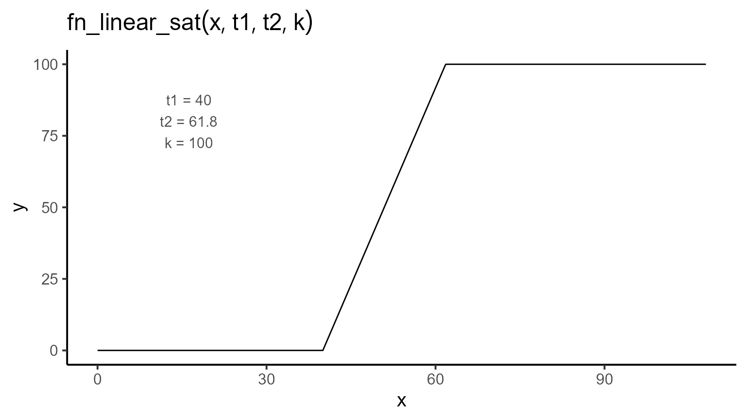
Once the data have been explored, we define the expectation function. In this case, it is a piece-wise regression function with three parameters: t1, t2, and k. The function can be expressed mathematically as follows:

fn_linear_sat()

\[\begin{equation} f(t; t_1, t_2, k) = \begin{cases} 0 & \text{if } t < t_1 \\ \dfrac{k}{t_2 - t_1} \cdot (t - t_1) & \text{if } t_1 \leq t \leq t_2 \\ k & \text{if } t > t_2 \end{cases} \end{equation}\]

plot fn

3. Fitting Models

To fit the model, we use the modeler function. Here:

x specifies the days after planting (DAP),
y is the canopy variable to be modeled,
grp allows us to perform group analysis, e.g., on multiple plots.

In this example, we have 196 plots but will only fit the model for plots 166 and 40 as a subset. We define the piecewise function fn_linear_sat and set initial values for the parameters.

mod_1 <- dt_potato |>
  modeler(
    x = DAP,
    y = Canopy,
    grp = Plot,
    fn = "fn_linear_sat",
    parameters = c(t1 = 45, t2 = 80, k = 0.9),
    subset = c(166, 40)
  )
mod_1
#> 
#> Call:
#> Canopy ~ fn_linear_sat(DAP, t1, t2, k) 
#> 
#> Sum of Squares Error:
#>     Min.  1st Qu.   Median     Mean  3rd Qu.     Max. 
#>  0.05448 10.26923 20.48397 20.48397 30.69871 40.91346 
#> 
#> Optimization Results `head()`:
#>  uid   t1   t2   k     sse
#>   40 34.8 60.6 100  0.0545
#>  166 31.6 57.5 100 40.9135
#> 
#> Metrics:
#>  Groups      Timing Convergence Iterations
#>       2 0.8338 secs        100% 558.5 (id)

After fitting, we can inspect the model summary and visualize the fit using the plot function:

plot(mod_1, id = c(166, 40))

plot fit

kable(mod_1$param)

uid	t1	t2	k	sse
40	34.84916	60.59505	100.0000	0.0544833
166	31.61374	57.54603	100.0047	40.9134555

3.1. Extracting model coefficients and uncertainty measures

Once the model is fitted, we can extract key statistical information, such as coefficients, standard errors, confidence intervals, and the variance-covariance matrix for each group (plot). These metrics allow us to draw conclusions about the parameter estimates and assess the uncertainty around them.

The functions coef, confint, and vcov are used as follows:

coef: Extracts the estimated coefficients for each group.
confint: Provides the confidence intervals for the parameter estimates.
vcov: Returns the variance-covariance matrix, which can be used to understand the relationships between the estimates and their variability.

coef(mod_1)
#> # A tibble: 6 × 6
#>     uid coefficient solution std.error `t value` `Pr(>|t|)`
#>   <dbl> <chr>          <dbl>     <dbl>     <dbl>      <dbl>
#> 1    40 t1              34.8    0.0240    1453.    2.93e-15
#> 2    40 t2              60.6    0.0368    1648.    1.56e-15
#> 3    40 k              100.     0.0603    1659.    1.51e-15
#> 4   166 t1              31.6    0.794       39.8   1.89e- 7
#> 5   166 t2              57.5    0.902       63.8   1.79e- 8
#> 6   166 k              100.     1.65        60.6   2.32e- 8

confint(mod_1)
#> # A tibble: 6 × 6
#>     uid coefficient solution std.error ci_lower ci_upper
#>   <dbl> <chr>          <dbl>     <dbl>    <dbl>    <dbl>
#> 1    40 t1              34.8    0.0240     34.8     34.9
#> 2    40 t2              60.6    0.0368     60.5     60.7
#> 3    40 k              100.     0.0603     99.8    100. 
#> 4   166 t1              31.6    0.794      29.6     33.7
#> 5   166 t2              57.5    0.902      55.2     59.9
#> 6   166 k              100.     1.65       95.8    104.

vcov(mod_1)
#> $`40`
#>               t1            t2            k
#> t1  5.755016e-04 -0.0002977975 4.429736e-08
#> t2 -2.977975e-04  0.0013525945 9.350853e-04
#> k   4.429736e-08  0.0009350853 3.632249e-03
#> 
#> $`166`
#>             t1         t2           k
#> t1  0.63072149 -0.2613850 -0.00283193
#> t2 -0.26138501  0.8131631  0.71197685
#> k  -0.00283193  0.7119768  2.72567110

4. Providing different initial values

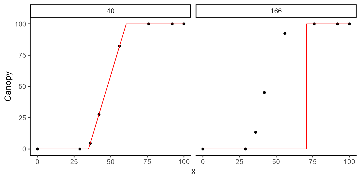
The initial fit may not always be optimal, so we can adjust the initial parameter values for each plot and even fix certain parameters to improve the model.

initials <- data.frame(
  uid = c(166, 40),
  t1 = c(70, 60),
  t2 = c(40, 80),
  k = c(100, 100)
)

kable(initials)

uid	t1	t2	k
166	70	40	100
40	60	80	100

mod_2 <- dt_potato |>
  modeler(
    x = DAP,
    y = Canopy,
    grp = Plot,
    fn = "fn_linear_sat",
    parameters = initials,
    subset = c(166, 40)
  )

plot(mod_2, id = c(166, 40))

plot fit 2

kable(mod_2$param)

uid	t1	t2	k	sse
40	34.84916	60.59505	100.0000	5.448330e-02
166	70.75697	39.85048	100.0047	1.077531e+04

It’s important to note that providing poor initial guesses for the parameters can lead to inaccurate or unreliable model fits. For example, if we mistakenly assign t1 (the day of plant emergence) a value greater than t2 (the day of maximum canopy), the model fit can fail or produce nonsensical results.

5. Fixing some parameters of the model

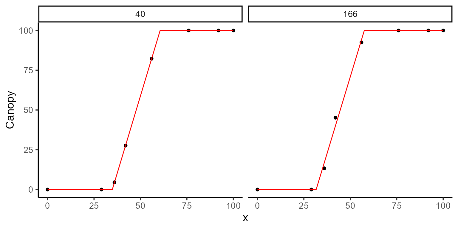
In certain cases, we may want to fix specific parameters either because they are known or because we prefer the model to leave these parameters unchanged. For example, we can fix the parameter k, which represents the maximum canopy value. If we assume that the maximum canopy coverage is 100%, we can incorporate this assumption into the model by fixing k.

fixed_params <- data.frame(uid = c(166, 40), k = c(100, 100))

kable(fixed_params)

uid	k
166	100
40	100

mod_3 <- dt_potato |>
  modeler(
    x = DAP,
    y = Canopy,
    grp = Plot,
    fn = "fn_linear_sat",
    parameters = c(t1 = 45, t2 = 80, k = 0.9),
    fixed_params = fixed_params,
    subset = c(166, 40)
  )

plot(mod_3, id = c(166, 40))

plot fit 3

kable(mod_3$param)

uid	t1	t2	sse	k
40	34.84916	60.59505	0.0544833	100
166	31.61374	57.54482	40.9135208	100

By fixing k to 100, we are telling the model that the maximum canopy for these plots is fixed at 100%. This allows the model to focus on estimating the other parameters, t1 and t2, potentially improving the accuracy of their estimates by reducing the complexity of the model.

6. Comparing estimations

rbind.data.frame(
  mutate(mod_1$param, model = "1", .before = uid),
  mutate(mod_2$param, model = "2", .before = uid),
  mutate(mod_3$param, model = "3", .before = uid)
) |>
  filter(uid %in% 166) |>
  kable()

model	uid	t1	t2	k	sse
1	166	31.61374	57.54603	100.0047	40.91346
2	166	70.75697	39.85048	100.0047	10775.31306
3	166	31.61374	57.54482	100.0000	40.91352

After fitting multiple models with different initial values, fixed parameters, and canopy adjustments, we can compare the resulting coefficients and sum of square errors (sse) to evaluate the impact of these changes.

rbind.data.frame(
  mutate(AIC(mod_1), model = "1", .before = uid),
  mutate(AIC(mod_2), model = "2", .before = uid),
  mutate(AIC(mod_3), model = "3", .before = uid)
) |>
  filter(uid %in% 166) |>
  kable()

model	uid	logLik	df	nobs	p	AIC
1	166	-17.87958	4	8	3	43.75916
2	166	-40.17379	4	8	3	88.34759
3	166	-17.87958	3	8	2	41.75917

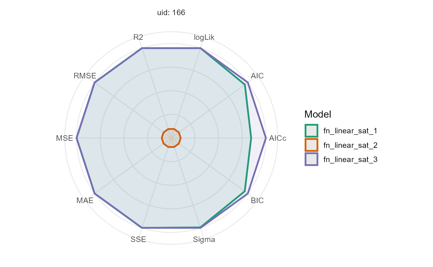
7. Making predictions

Once the model is fitted and validated as the best representation of our data, we can proceed to make predictions. The predict.modeler() function provides a range of flexible prediction options, allowing users to perform point predictions, calculate the area under the curve (AUC), compute first or second derivatives, and even evaluate custom functions of the parameters. Below are some examples demonstrating these capabilities:

# Point Prediction
predict(mod_1, x = 45, type = "point", id = 166) |> kable()

uid	x_new	predicted.value	std.error
166	45	51.62246	1.656734

# AUC Prediction
predict(mod_1, x = c(0, 108), type = "auc", id = 166) |> kable()

uid	x_min	x_max	predicted.value	std.error
166	0	108	6342.308	93.61781

# Function of the parameters
predict(mod_1, formula = ~ t2 - t1, id = 166) |> kable()

uid	formula	predicted.value	std.error
166	t2 - t1	25.93229	1.402375

In each example, the predict.modeler() function tailors the predictions to the user’s needs, whether it’s estimating a single value, integrating across a range, or calculating a parameter-based expression.

8. Modelling all plots using parallel processing

Finally, we can apply this method to all 196 plots, leveraging parallel processing to speed up the computation. To do this, we specify parallel = TRUE in the options argument, and set the number of cores using the function parallel::detectCores(), which automatically detects the available cores.

explorer <- explorer(dt_potato, x = DAP, y = Canopy, id = Plot)
fixed_params <- explorer |>
  pluck("dt_long") |>
  filter(var %in% "Canopy") |>
  group_by(uid) |>
  summarise(k = max(y), .groups = "drop")
mod <- dt_potato |>
  modeler(
    x = DAP,
    y = Canopy,
    grp = Plot,
    fn = "fn_linear_sat",
    parameters = c(t1 = 45, t2 = 80, k = 0.9),
    fixed_params = fixed_params,
    options = list(progress = TRUE, parallel = TRUE, workers = 5)
  )