Select the best model for each group

Compares two or more fitted modeler objects and selects the preferred model separately for each group (uid). Candidate models are ranked using one or more model-performance metrics.

Usage

model_selection(..., metrics = "AICc", return_table = FALSE)

Arguments

...: Two or more model objects (only of class modeler), fitted on the same groups.
metrics: Character vector specifying the metrics used for model selection. Available options are "logLik", "AIC", "AICc", "BIC", "Sigma", "SSE", "MAE", "MSE", "RMSE", and "R2". Use "all" to include all available metrics. The default is "AICc".
return_table: Logical. If TRUE, the selection table is returned instead of the combined modeler object. FALSE by default.

Value

A modeler object holding the winning fit for each group. Two attributes are attached: "selection" (the winner, its score and the number of metrics used, per group) and "performance" (the full comparison table, of class performance, ready for plot()).

Details

Model selection is performed independently within each group. For each metric, candidate models are min-max rescaled to a range from 0.1 to 1. Metrics for which smaller values indicate better performance (AIC, AICc, BIC, Sigma, SSE, MAE, MSE, and RMSE) are reversed after rescaling, whereas logLik and R2 retain their original direction. Higher rescaled values therefore always indicate better performance.

Several available metrics contain overlapping information. For example, SSE, MSE, RMSE, and R2 produce equivalent rankings within a group, while AIC, AICc, and BIC are all likelihood-based criteria that differ in how model complexity is penalized. Consequently, metrics = "all" should not be interpreted as combining independent measures of model performance. When multiple metrics are used, an explicit subset should be chosen according to the objective of the analysis.

Author

Johan Aparicio [aut]

Examples

library(flexFitR)
data(dt_potato)
mod_1 <- dt_potato |>
  modeler(
    x = DAP,
    y = Canopy,
    grp = Plot,
    fn = "fn_lin_plat",
    parameters = c(t1 = 45, t2 = 80, k = 90),
    subset = c(1, 7)
  )
mod_2 <- dt_potato |>
  modeler(
    x = DAP,
    y = Canopy,
    grp = Plot,
    fn = "fn_logistic",
    parameters = c(a = 0.199, t0 = 47.7, k = 100),
    subset = c(1, 7)
  )
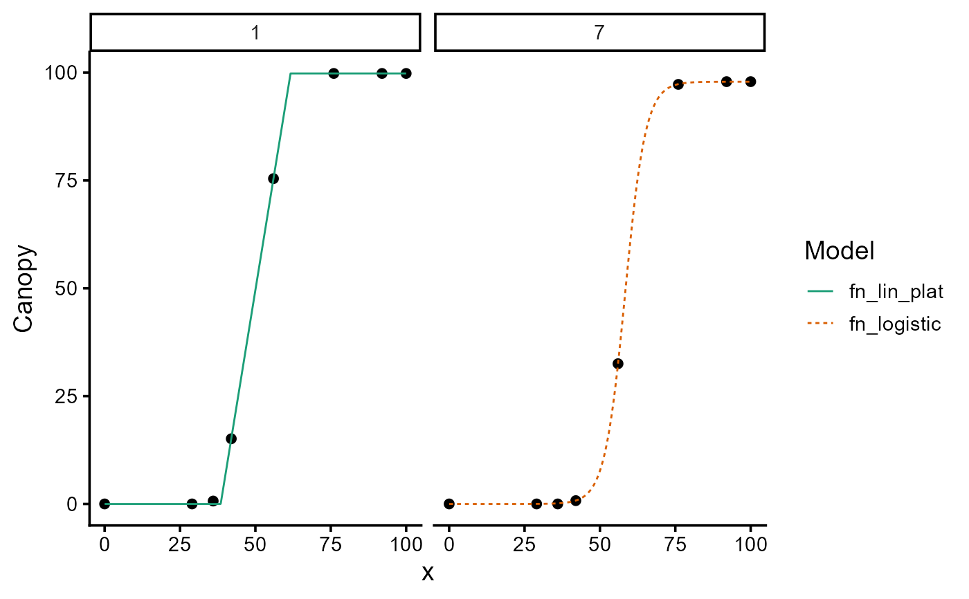
best <- model_selection(mod_1, mod_2, metrics = "AIC")
print(best)
#> 
#> Call:
#> Canopy ~ fn_lin_plat(DAP, t1, t2, k) | uid (1) 
#> Canopy ~ fn_logistic(DAP, a, t0, k) | uid (1) 
#> 
#> Residuals (`Standardized`):
#>     Min.  1st Qu.   Median     Mean  3rd Qu.     Max. 
#> -1.92280 -0.06156  0.00000 -0.01653  0.01173  2.23607 
#> 
#> Optimization Results `head()`:
#>  uid coefficient solution std.error t value Pr(>|t|)
#>    1          t1   38.492   0.08871   433.9 1.23e-12
#>    1          t2   61.661   0.10929   564.2 3.32e-13
#>    1           k   99.811   0.17299   577.0 2.97e-13
#>    7           a    0.294   0.00495    59.4 2.57e-08
#> 
#> Metrics:
#>  Groups Timing Convergence Iterations
#>       2 0.5269        100% 575.5 (id)
#> 
attr(best, "selection")
#> # A tibble: 2 × 6
#>     uid fn_name       score n_metrics model       order
#>   <dbl> <chr>         <dbl>     <int> <chr>       <int>
#> 1     1 fn_lin_plat_1     1         1 fn_lin_plat     1
#> 2     7 fn_logistic_2     1         1 fn_logistic     2
plot(best, id = c(1, 7))